Graphing#
The picture is a model of reality. - Ludwig Wittgenstein
In this lab, you will get familiar with the statistical plotting features of Python using several famous datasets from the history of science.
Instructions#
Create a folder named LASTNAME_FIRSTNAME_project_one, replacing LASTNAME and FIRSTNAME with your last name and first name, respectively.
Download both csv datasets in the Velocity of Light section and place it in the new folder you created in step 1.
In the same folder, create a Python py script named project_one.py.
Create a Python docstring at the very top of the script file. Keep all written answers in this area of the script.
Read the Background section and the Loading In Data section.
Perform all exercises and answer all questions in the Project section. Label your script with comments as indicated in the Project section.
When you are done, zip your folder and all its contents into a file named LASTNAME_FIRSTNAME_project_one.zip
Upload the zip file here: TODO
Tip
You may need to refer to the Plots page for examples of various types of graphs.
Formulae#
Recall the formula for percent error is given by,
Background#
The Michelson Velocity of Light Experiment#
The Michelson Velocity of Light Experiment<https://www.gutenberg.org/files/11753/11753-h/11753-h.htm> conducted in 1887 was a landmark experiment for severals reason.
TODO
remained one of most accurate estimations of the speed of light until modern times. Using a series of mirrors depicted below,
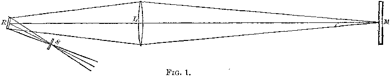
He was able to measure the fractional time difference in lights of ray arriving
TODO
While the theoretical details of the experiment are interesting in their own right (see link above for further detail!), for this lab, we will take the data as given and analyze it from a statistical perspective.
The Cavendish Density of the Earth Experiment#
Henry Cavendish performed the first modern, scientific experiment to measure the density of the Earth in 1797. Using the mutual gravitational attraction of two heavy metal balls attached to a torsion balanace to twist a fiber of string, Cavendish measured the force of the tension produced. With Newton’s Laws of Motion , he was able to derive an expression that related this force to the mass of the Earth.
The estimate produced by Cavendish remained until modern times one of the most accurate and authoritative measures of the Earth’s mass. In this lab, we will analyze the data produced by Cavendish.
Loading In Data#
The following code snippet will load in a CSV spreadsheet named example.csv, parse it into a list and then print it to screen, assuming that CSV file is saved in the same folder as your script. Modify this code snippet to fit the datasets in this lab and then use it to load in the provided datasets in Velocity of Light section.
import csv

# read in data
with open('example.csv') as csv_file:
    csv_reader = csv.reader(csv_file)
    raw_data = [ row for row in csv_reader ]

# separate headers from data
headers = raw_data[0]
columns = raw_data[1:]

# grab first column from csv file and ensure it's a number (not a string)
column_1 = [ float(row[0]) for row in columns ]

print(column_1)
Project#
Velocity of Light#
Load the Velocity of Light data into a Python Script using the tecnique outlined in the Loading In Data section.
Construct a histogram plot for this data sets using eight classes. Answer the following questions in the body of your docstring.
What is the class width of your histogram?
What are the class limits for each class?
What is the most frequent class?
What type of shape does this distribtion have? Is this expected? Why or why not?
Construct a boxplot for this data set. Using the boxplot, answer the following questions in the body of your docstring.
Estimate the 75 th percentile of this data set.
Estimate the 25 th percentile of this data set.
Estimate the median of this data set.
Estimate the range of this data set.
The actual value of the speed of light, according to the best estimates we have today, is
 . Use this information to answer the following questions in the body of your docstring.
What is the sample mean of the dataset?
What is the percent error of this estimate with respect to the actual value.
Density of the Earth#
Load the Density of the Earth data into a Python Script using the tecnique outlined in the Loading In Data section.
Construct a histogram plot for this data sets using eight classes. Answer the following questions in the body of your docstring.
What is the class width of your histogram?
What are the class limits for each class?
What is the most frequent class?
What type of shape does this distribtion have? Is this expected? Why or why not?
Construct a boxplot for this data set. Using the boxplot, answer the following questions in the body of your docstring.
Estimate the 75 th percentile of this data set.
Estimate the 25 th percentile of this data set.
Estimate the median of this data set.
Estimate the range of this data set.
The actual value of the speed of light, according to the best estimates we have today, is
 . Use this information to answer the following questions in the body of your docstring.
What is the sample mean of the dataset?
What is the percent error of this estimate with respect to the actual value?
Datasets#
Velocity of Light Data#
You can download the full dataset here.
The following table is the a preview of the data you will be using for this project.
Velocity ( km/s ) |
299850 |
299740 |
299900 |
300070 |
299930 |
299850 |
299950 |
299980 |
The meaning of the column is clear from the column header: each observation measures the speed of light in meters per second,  .
.
Density of the Earth Data#
You can download the full dataset here.
The following table is the a preview of the data you will be using for this project.
Experiment Density |
1 5.5 |
2 5.61 |
3 4.88 |
4 5.07 |
5 5.26 |
6 5.55 |
7 5.36 |
8 5.29 |
9 5.58 |
10 5.65 |
11 5.57 |
The first column corresponds to the experiment number (first, second, third, etc.). The second column is the ratio of the density of Earth to the density of water. Recall the density of water by definition is  .
.