STATPLOT: Binomial Histogram#

Introduction#

Previously, we have introduced the two main functions for working with Binomial Random Variables. We took a look at the BINOMPDF, the probability density function, and the BINOMCDF, the cumulative distribution function, for a Binomial Random Variable. In this section, we will use these functions again to create visualizations for different Binomial Random Variables.

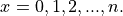
Recall the Binomial Random Variable counts the number of successes in a fixed number of independent trials, where a success occurs with probability ``p`` and a failure occurs with probability 1-p. Furthermore, the probability of a success is the same across all trials. The probability density function for a Binomial Random Variable is given by,

$P(\mathcal{X} = x) = C(n,x) \cdot p^x \cdot (1-p)^{n-x}$

Note the domain of this function is given by,

$x = 0, 1, 2, ..., n.$

In other words, the Binomial PDF is only defined for integer values of x from 0 up to n. For any values of x outside of this range, the Binomial PDF is undefined.

Calculator#

Recall the Binomial PDF can be accessed on your calculator as follows,

Let us use this function to explore how the parameters of a Binomial Random Variable affect the shape of its distribution. The two parameters of a Binomial Random Variable are,

``n``: The number of trials.
``p``: The probability of success.

Activity#

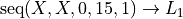
Let us fix $n=15$ . To start, we will need to generate a list that represents the domain of the Binomial Random Variable. Go to the STAT editor and select the formula bar for $L_1$ . Use the SEQ editor to generate a list of numbers from 0 to 15,

$\text{seq}(X, X, 0, 15, 1) \rightarrow L_1$

Question #1

Just to verify you are following along: What is $\text{sum}(L_1)$ ?

Now that we have the domain of our Binomial Random Variable in $L_1$ , let’s look at its PDF for various values of p. Let’s start with $p=0.5$ .

Go to the STAT editor and select the formula bar for $L_2$ and enter the following formula,

$\text{binompdf}(15, 0.5, L_1)$

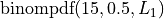
Execute the formula and will be populated by the values of the Binomial PDF corresponding to the inputted elements of the domain in :math:L_1.

Use $L_1$ and $L_2$ to generate a histogram of this Binomial Distribution. Ensure you have your view WINDOW set to the following dimenions and scale,

Xmin: 0 Xmax: 16 Xscl: 1 Ymin: 0 Ymax: 0.5

Question #2

What is the expected value fo the Distribution with $n=15$ and $p=0.5$ ?
What is the median of the Binomial Distribution with $n=15$ and $p=0.5$ ?
What is the standard deviation fo the Binomial Distribution with $n=15$ and $p=0.5$ ? Round to three decimal places.
Write a few sentences describing the Binomial Distribution with $n=15$ and $p=0.5$ .

Now, using the same technique, generate a new list in $L_3$ that represents the Binomial Distribution when $p=0.25$ .

Question #3

What is the expected value fo the Distribution with $n=15$ and $p=0.25$ ?
What is the median of the Binomial Distribution with $n=15$ and $p=0.25$ ?
What is the standard deviation of the Binomial Distribution with $n=15$ and $p=0.25$ ?

Again, using the same technique, generate a new lsit in in $L_4$ that represents the Binomial Distribution when $p=0.75$ .

Question #4

What is the expected value fo the Distribution with $n=15$ and $p=0.75$ ?
What is the median of the Binomial Distribution with $n=15$ and $p=0.75$ ?
What is the standard deviation of the Binomial Distribution with $n=15$ and $p=0.75$ ?

Question #5

Write a few sentences comparing and contrasting the three Binomial Distributions you have created. How does changing the probability of success affect the shape, center and variation of the Binomial Distribution?

Solutions#

TODO: jquery these into hidden elements

1: 120
2a: 7.5
2b: 7.5
2c: 1.936
3a: 3.75
3b: 4
3c: 1.677
4a: 11.25
4b: 11
4c: 1.677

STATPLOT: Binomial Histogram

Contents

STATPLOT: Binomial Histogram#

Introduction#

Calculator#

Activity#

Solutions#