Data#

Classifications#

The data we collect from an experiment is classified according to several factors.

Dimensionality#

Definition

The dimension of a dataset is the number of values associated with a single observation.

Univariate: $\{ x_1, x_2, x_3 \}$

Univariate data consists of observations that each contain a single value.

Example: Experimental data from Henri Cavendish’s density of the Earth experiments. Density is expressed as a ratio of the density of water. See Bar Charts for more information about this dataset.

Density of the Earth#
Density
5.5
5.61
4.88
5.07
5.26
5.55
5.36
5.29
5.58
5.65
5.57

Bivariate: $\{ (x_1, y_1), (x_2, y_2), ... , (x_n, y_n)\}$

Bivariate data consists of observations that each contain two values (i.e. an pair)

Example: Data from the Challenger space shuttle explosion showing the atmospheric temperature versus the erosion index of the O-ring seal. The failure of the O-ring seal at lower temperatures was not accounted for prior to launch.

Challenger Space Shuttle Erosion Data#
Temp	Erosion
66.0	0.0
70.0	53.0
69.0	0.0
68.0	0.0
67.0	0.0
63.0	0.0
70.0	28.0
78.0	0.0
67.0	0.0

Multivariate: $\{ (x_{1}^1, x_{2}^1, ... , x_{n}^1 ), (x_{1}^2, x_{2}^2, ... , x_{n}^2 ), ... ,(x_{1}^m, x_{2}^m, ... , x_{n}^m )$

Multivariate data consists of observations that each contain an arbitrary number of values (i.e. a vector)

Example: Body measurements from a sample of grizzly bears.

Bear Measurements#
AGE	MONTH	SEX (1=M)	HEADLEN	HEADWDTH	NECK	LENGTH	CHEST	WEIGHT
19	7	1	11.0	5.5	16.0	53.0	26.0	80
55	7	1	16.5	9.0	28.0	67.5	45.0	344
81	9	1	15.5	8.0	31.0	72.0	54.0	416
115	7	1	17.0	10.0	31.5	72.0	49.0	348
104	8	0	15.5	6.5	22.0	62.0	35.0	166

Characteristic#

Definition: The characteristic of a dataset is the type of data being observed.
Qualitative: $\{ \text{red}, \text{blue}, \text{yellow} \}$

Qualitative data are categorical.

Example

The favorite color of a sample of people.
A group of people’s answer to supporting a new tax reform law.
Movies that feature Kevin Bacon.
Words that appear in a novel.

Quantitative

Quantitative data are numerical.

These are two types of quantitative data, discrete and continuous.

Discrete Quantitative: $\{ 1, 2, 3, 4, 5, ... \}$

Discrete quantitative data are countable.

Example

Students in a class.
Petals on a clover
The championships won by a football team.
M&M’s in a bag.

Continuous Quantitative

$\{ 1.0, 1.01, 1.001, 1.0001, 1.00001, ... \}$

Continuous quantitative data are infinitely divisible

Example

The temperature of a gallon of water under various pressures.
The speed of a train.
The weight of a coin.
The amount of rainfall in a region.

Scale#

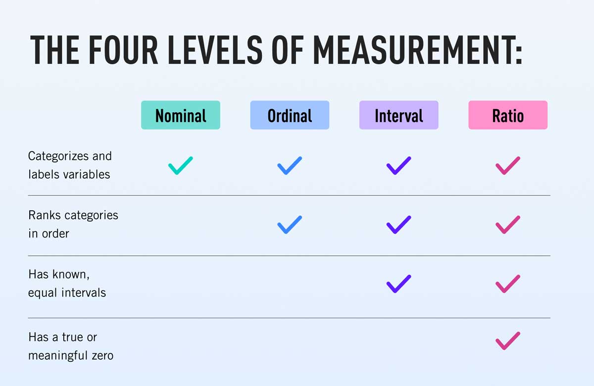
Nominal Level: Unordered, categorical data.

Nominal data is the simplest type of data. A nominal scale or level is a way of labelling and separating individuals in a sample into groups.

Example

The favorite color of each person in a sample of data.
The political party affiliation of each person in a sample of data.
The nationality of each person in a sample of data.

Ordinal Level

Ordered, categorical data.

Ordinal data is a step above nominal data. It is categorical, but an order can be imposed on it.

Example

Answers to a customer satisfaction survey: DISSATISFIED, NEUTRAL, SATISIFED
Grades on a quiz: A, B, C, D, E, F.

Interval Level

Ordered, numerical data.

Interval level is a step above ordinal data. The data are ordered, but now the difference between observations is defined. In other words, with an interval level, the distance between two observation $x_2$ and $x_1$ can be defined as $x_2 - x_1$

Example

A historical time series of the Consumer Price Index
The IQs of a random sample of people.
The SAT scores of the graduating class of seniors.

Ratio Level

Ordered, numerical data.

Ratio level is the final level of data. The data are ordered, the difference between two datapoints can be computed $x_2 - x_1$ and there is a true zero. With a ratio level, it makes sense to have an observation of 0.

Example

Measurements from a scale, i.e. the weight of a mass.
Measurements from a thermometer, i.e the temperature of a body.
The amount of rainfall in a region over a period of a week.

Types of Statistics#

Sample Statistic: A piece of information calculated from sample of data.

Sample statistics are used to summarize the features of a dataset. They are broken down into two main categories.

Descriptive Statistic: A sample statisic used to visualize and approximate the shape and spread of a population.

Inferential Statistic: A sample statistic used to make inferences about the population.

One of the most important descriptive statistics is the sample mean,

$\bar{x} = \frac{ \sum^n_{i = 1} x_i } {n}$

One of the most important inferential statistics is the Z-score of the sample mean,

$Z = \frac{ \bar{x} - \mu }{ \frac{ \sigma }{\sqrt n} }$

If these formulae make no sense yet, don’t worry! That is to be expected. They are listed here, so you can start forming a picture of the things to come. By the end of this class, these two formulae will become your best friends.

Data

Contents

Data#

Classifications#

Dimensionality#

Characteristic#

Scale#

Types of Statistics#